Health Costs Calculator

Jan 4, 2024

freeCodeCamp Machine Learning Certification

keras machine learning ml python regression tensorflow

Intro

This is the fourth project in the freeCodeCamp Machine Learning with Python Certification. For this project we have to create a book recommendation engine using K-Nearest Neighbors. We can use Tensorflow and scikit-learn to build our model. We will use the boilerplate code provided by freeCodeCamp. The Read more about it in Linear Regression Health Costs Calculator.

Check out the full code for this project at https://colab.research.google.com/drive/1gO9UJpHcYH04fEK4wMZ9R9N-6c9PLX4g?usp=sharing

Planning

For this project we will use linear regression algorithm. We can implement the algorithm using Keras sequential model with a single Dense with output size of one. Before training the model, we have to get our data ready for it.

We will use Pandas DataFrame to import the health costs data. We will check the data to make sure there are no missing or incorrect values, convert the categorical data to numeric data and filter the data if needed. We will format the data so it can be used with linear regression model. We will then do a 80-20 train-test split. We will also normalize our numerical data by adding a normalizer layer to our model.

Code

Let’s start by downloading the data we need. Run in shell

wget https://cdn.freecodecamp.org/project-data/health-costs/insurance.csv

Now in our python project, import the libraries we need

import numpy as np
import pandas as pd

import tensorflow as tf

from tensorflow import keras
from tensorflow.keras import layers

Data

Read the data to a Pandas DataFrame and check what it looks like

df = pd.read_csv('insurance.csv')
df.tail()

	age	sex	bmi	children	smoker	region	expenses
1333	50	male	31.0	3	no	northwest	10600.55
1334	18	female	31.9	0	no	northeast	2205.98
1335	18	female	36.9	0	no	southeast	1629.83
1336	21	female	25.8	0	no	southwest	2007.95
1337	61	female	29.1	0	yes	northwest	29141.36

df.describe()

	age	bmi	children	expenses
count	1338.000000	1338.000000	1338.000000	1338.000000
mean	39.207025	30.665471	1.094918	13270.422414
std	14.049960	6.098382	1.205493	12110.011240
min	18.000000	16.000000	0.000000	1121.870000
25%	27.000000	26.300000	0.000000	4740.287500
50%	39.000000	30.400000	1.000000	9382.030000
75%	51.000000	34.700000	2.000000	16639.915000
max	64.000000	53.100000	5.000000	63770.430000

df.shape

(1338, 7)

Check if there are any incorrect values

df.sex.unique()

array(['female', 'male'], dtype=object)

df.smoker.unique()

array(['yes', 'no'], dtype=object)

df.region.unique()

array(['southwest', 'southeast', 'northwest', 'northeast'], dtype=object)

Check if there are any missing values

df.isna().sum()

age         0
sex         0
bmi         0
children    0
smoker      0
region      0
expenses    0
dtype: int64

Our data looks clean. There are no missing values or typos in categorical values. Let’s format the data for use with our model.

For categorical data, we should use one hot encoding instead of converting to enumerated type because we are using regression and the enumerated values might not have a linear relation with the health costs.

We will one hot encode the children column too because we are not sure if there is a linear relation between the number of children and health costs. We will also add categories for age and BMI for the same reason.

One hot encode the sex column and drop it after. This will add two columns, female and male.

df = df.join(pd.get_dummies(df.sex))
df = df.drop('sex', axis=1)
df

	age	bmi	children	smoker	region	expenses	female	male
0	19	27.9	0	yes	southwest	16884.92	1	0
1	18	33.8	1	no	southeast	1725.55	0	1
2	28	33.0	3	no	southeast	4449.46	0	1
3	33	22.7	0	no	northwest	21984.47	0	1
4	32	28.9	0	no	northwest	3866.86	0	1
…	…	…	…	…	…	…	…	…
1333	50	31.0	3	no	northwest	10600.55	0	1
1334	18	31.9	0	no	northeast	2205.98	1	0
1335	18	36.9	0	no	southeast	1629.83	1	0
1336	21	25.8	0	no	southwest	2007.95	1	0
1337	61	29.1	0	yes	northwest	29141.36	1	0

Similarly, one hot encode children, smoker and region columns

df = df.join(pd.get_dummies(df.smoker, prefix='smoker'))
df = df.drop('smoker', axis=1)

df = df.join(pd.get_dummies(df.region, prefix='region'))
df = df.drop('region', axis=1)

df = df.join(pd.get_dummies(df.children, prefix='children'))
df = df.drop('children', axis=1)

We can’t create one hot encoding for age and bmi directly since they are numeric values. We will use bins and labels to encode the data

df['overweight'] = df.bmi > 30
df = df.join(pd.get_dummies(df.overweight, prefix='overweight'))
df = df.drop('overweight', axis=1)

df = df.join(pd.get_dummies(pd.cut(df['bmi'], bins=[0,18,25,30,100], labels=['w_low', 'w_normal', 'w_heigh', 'w_over'])))

df = df.join(pd.get_dummies(pd.cut(df['age'], bins=[10,25,35,45,55,60,100], labels=['yt25', 'yt35', 'yt45', 'yt55', 'yt60', 'o60'])))
df.head()

	age	bmi	expenses	female	male	smoker_no	smoker_yes	region_northwest	region_southeast	region_southwest	overweight_False	overweight_True	w_normal	w_heigh	w_over	children_0	children_1
0	19	27.9	16884.92	1	0	0	1	0	0	1	1	0	0	1	0	1	0
1	18	33.8	1725.55	0	1	1	0	0	1	0	0	1	0	0	1	0	1
2	28	33.0	4449.46	0	1	1	0	0	1	0	0	1	0	0	1	0	0
3	33	22.7	21984.47	0	1	1	0	1	0	0	1	0	1	0	0	1	0
4	32	28.9	3866.86	0	1	1	0	1	0	0	1	0	0	1	0	1	0

Training

Create the training and testing DataFrames

train_dataset = df.sample(frac=0.8)
test_dataset = df.drop(train_dataset.index)

train_labels = train_dataset.pop('expenses')
test_labels = test_dataset.pop('expenses')

train_dataset.shape
(1070, 28)

test_dataset.shape
(268, 28)

We can start creating our model now

model = keras.Sequential()

Create a normalization layer and pass it the mean and variance using its adapt method. Then add it to our model

normalizer = layers.Normalization(axis=-1)
normalizer.adapt(np.array(train_dataset))

model.add(normalizer)

Add one Dense layer with one unit

model.add(layers.Dense(1))

Compile the model. We will use the Adam for optimizer, mean absolute error for loss function and mean absolute error and mean square error for metrics

model.compile(optimizer=keras.optimizers.Adam(learning_rate=5.0),
              loss='mae', metrics=['mae', 'mse'])

model.build()
model.summary()

Model: "sequential"
_________________________________________________________________
 Layer (type)                Output Shape              Param #   
=================================================================
 normalization (Normalizati  (None, 28)                57        
 on)                                                             
                                                                 
 dense (Dense)               (None, 1)                 29        
                                                                 
=================================================================
Total params: 86 (348.00 Byte)
Trainable params: 29 (116.00 Byte)
Non-trainable params: 57 (232.00 Byte)
_________________________________________________________________

Train the model for 400 steps

history = model.fit(
    train_dataset, train_labels,
    epochs=400,
    validation_split = 0.2,
    )

Epoch 1/400
27/27 [==============================] - 2s 24ms/step - loss: 12980.1807 - mae: 12980.1807 - mse: 310381984.0000 - val_loss: 13748.0254 - val_mae: 13748.0254 - val_mse: 346313440.0000
Epoch 2/400
27/27 [==============================] - 0s 8ms/step - loss: 12835.0674 - mae: 12835.0674 - mse: 307191456.0000 - val_loss: 13636.8164 - val_mae: 13636.8164 - val_mse: 343705664.0000
Epoch 3/400
27/27 [==============================] - 0s 5ms/step - loss: 12694.8037 - mae: 12694.8037 - mse: 303253088.0000 - val_loss: 13522.0586 - val_mae: 13522.0586 - val_mse: 340197760.0000
Epoch 4/400
27/27 [==============================] - 0s 10ms/step - loss: 12555.8711 - mae: 12555.8711 - mse: 299622240.0000 - val_loss: 13407.2188 - val_mae: 13407.2188 - val_mse: 337578304.0000
...
27/27 [==============================] - 0s 3ms/step - loss: 3059.3418 - mae: 3059.3418 - mse: 46594180.0000 - val_loss: 3746.8494 - val_mae: 3746.8494 - val_mse: 58849572.0000
Epoch 398/400
27/27 [==============================] - 0s 4ms/step - loss: 3059.8738 - mae: 3059.8738 - mse: 46530496.0000 - val_loss: 3750.7312 - val_mae: 3750.7312 - val_mse: 58936692.0000
Epoch 399/400
27/27 [==============================] - 0s 4ms/step - loss: 3058.9065 - mae: 3058.9065 - mse: 46630444.0000 - val_loss: 3750.1858 - val_mae: 3750.1858 - val_mse: 59066800.0000
Epoch 400/400
27/27 [==============================] - 0s 5ms/step - loss: 3061.2319 - mae: 3061.2319 - mse: 46695008.0000 - val_loss: 3757.2839 - val_mae: 3757.2839 - val_mse: 58933712.0000

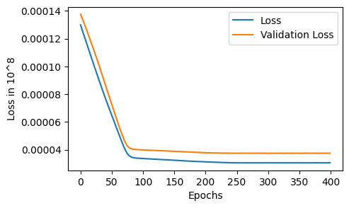
Plot the loss and validation loss

fig, axes = plt.subplots(figsize=(5,3))
axes.plot(np.array(history.history['loss'])/10**8)
axes.plot(np.array(history.history['val_loss'])/10**8)
axes.set_xlabel('Epochs')
axes.set_ylabel('Loss in 10^8')
axes.legend(['Loss', 'Validation Loss'])

Loss

Testing

Time to test our model and see if it passed the freeCodeCamp requirements

NOTE: This code block is provided by freeCodeCamp

loss, mae, mse = model.evaluate(test_dataset, test_labels, verbose=2)

print("Testing set Mean Abs Error: {:5.2f} expenses".format(mae))

if mae < 3500:
  print("You passed the challenge. Great job!")
else:
  print("The Mean Abs Error must be less than 3500. Keep trying.")

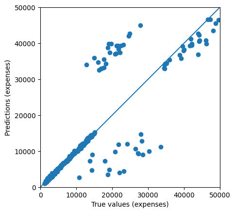
# Plot predictions.
test_predictions = model.predict(test_dataset).flatten()

a = plt.axes(aspect='equal')
plt.scatter(test_labels, test_predictions)
plt.xlabel('True values (expenses)')
plt.ylabel('Predictions (expenses)')
lims = [0, 50000]
plt.xlim(lims)
plt.ylim(lims)
_ = plt.plot(lims,lims)

9/9 - 0s - loss: 3199.8831 - mae: 3199.8831 - mse: 49219736.0000 - 53ms/epoch - 6ms/step
Testing set Mean Abs Error: 3199.88 expenses
You passed the challenge. Great job!
9/9 [==============================] - 0s 2ms/step

Predictions

We have less than $3200 MSE and passed the challenge!

Thank you for reading. You can also check out my other projects for this series below.